The FIRE math looks simple from the outside: save aggressively, invest, and quit when your portfolio reaches roughly 25 times your annual spending. The hard part is that the answer to "when" is a distribution, not a date — it depends on the order in which markets deliver returns, and nobody controls that. A calculator that draws one smooth, average-return line across your future is quietly hiding the only part of the picture that matters.
The financial independence simulator is a free FIRE calculator that runs the honest version of that math in your browser. It takes your assets, debts, income, and spending; produces a year-by-year net-worth projection; dates your FI and RE milestones; adds a seeded Monte Carlo success rate; and lets you compare scenarios side by side, with every number recomputing live as you type. Your plan saves as a JSON file, so the numbers survive the tab closing.
Try Financial Independence Simulator — free, no sign-up.
This post covers what each piece of the simulation actually means — sequence-of-returns risk in plain words, which inputs move your date the most, how to read a percentile chart — and where the honest limits of any model sit. For the underlying arithmetic, the FIRE math explained guide is the companion read.
What a FIRE calculator actually computes
The core loop is one recurrence, repeated per year: net worth grows by the assumed return plus new savings, and shrinks by spending and any debt costs. Run it forward for decades and the simulator can date two distinct events. FI — financial independence — is when net worth first crosses your target, conventionally 25 times annual spending under the 4 percent rule lineage. RE — retire early — is the date you actually stop working, which you set yourself. Plenty of people keep working past FI; plenty of others coast in the middle ground where saved capital finishes the job on its own, which is the territory covered in the coast FIRE guide.
The simulator's inputs map directly onto that recurrence: current assets, debts, income, and spending. Everything recomputes live — nudge spending upward and the FI date, the RE date, and the whole projection move immediately. That live feedback is not a convenience feature; it is how you learn which inputs actually matter, because you watch the consequences instead of imagining them.
Why average returns lie: sequence-of-returns risk
Two portfolios can experience the exact same average return over the same period and end up in genuinely different places. The reason is the single most important concept in retirement math, and it takes a five-year toy example to see it.
Take a $100,000 portfolio that withdraws $4,000 at the start of each year. Both return sequences below average exactly 6 percent per year — identical sums, different order:
| Year | Path A return | Path A balance | Path B return | Path B balance |
|---|---|---|---|---|
| 1 | +30% | $124,800 | −20% | $76,800 |
| 2 | +10% | $132,880 | +5% | $76,440 |
| 3 | −20% | $103,104 | +5% | $76,062 |
| 4 | +5% | $104,059 | +10% | $79,268 |
| 5 | +5% | $105,062 | +30% | $97,848 |
Identical averages, a $7,200 gap at the end — and Path B never visibly catches up despite the identical boom-and-bust inventory. The mechanism: when money is flowing out every year, losses early in retirement are suffered from a larger base, and the later boom arrives to compound a smaller one. Stretch this from five years to forty, scale withdrawals from 4 percent to a FIRE-level drawdown, and the order of returns alone can decide whether a plan survives. This is sequence-of-returns risk, and it is why a safe withdrawal rate simulator worth using cannot be a single line.
What Monte Carlo adds, and what "seeded" means
Monte Carlo replaces the one smooth path with many randomized ones. For each simulated future, the calculator draws a long sequence of returns — good years, bad years, crashes, booms, in random order — and runs your complete plan through it: contributions while working, withdrawals after, the works. Then it does it again, many times over. The success rate is the share of those futures in which your money never runs dry before the horizon you set.
"Seeded" means the random draws start from a value you can repeat. Run the same plan twice and you get the same set of futures, which sounds like a nitpick until you try to compare scenarios: with an unseeded simulator, a change in the success rate might reflect your new input or might just be a fresh roll of the dice. With a seeded one, identical inputs give identical results, so any movement in the number is caused by the thing you changed. Small implementation detail, large difference in what the tool can honestly tell you.
How to read a percentile fan chart
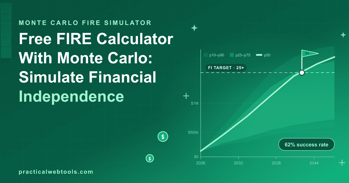
Instead of one line, a Monte Carlo projection shows a fan of outcome bands, typically labeled by percentile:
| Band | What it means | What to do with it |
|---|---|---|
| p90 (optimistic tail) | Strong markets; money was never the constraint | Do not plan around it |
| p50 (median) | The middle future | A useful reference, not a promise |
| p10 (pessimistic tail) | Poor sequencing — the plan's stress case | This band should fund your decisions |
The discipline that separates useful simulation from wallpaper: read the p10 band, not the p50 line. If the tenth-percentile path still clears your horizon, the plan is robust. If it depletes at 78 while you modeled living to 95, you have found the weakness while it is still cheap to fix — and the fix levers, roughly in order of impact, are spending, income, and retirement date.
The inputs that move the date the most
Not all inputs are equal, and live recompute makes the ranking visible in seconds. In testing the simulator, raising annual spending from $48,000 to $70,000 — changing nothing else — moved the FI age from 62 to 70 and dropped the Monte Carlo success rate from 62 percent to 34 percent. One input: eight years of working, and the difference between "probably fine" and "coin flip."
The two effects compound. Under the 25-times convention, those spending levels imply FI targets of $1.2 million versus $1.75 million, so the date has to slip just to reach the bigger number. But the success rate falls faster than the date slips, because higher withdrawals make the same portfolio more fragile to bad return sequencing — spending more does not just mean needing more, it means the plan bends sooner when markets arrive in the wrong order.
The other high-leverage inputs, in rough order: your assumed returns, which you choose and which the model will faithfully believe; your income trajectory, since the savings rate is the engine of the entire projection; and debts, which behave like negative returns for as long as they last.
A five-minute run-through
- Enter assets and debts. Everything that compounds for you, and everything that compounds against you.
- Enter income and spending. Be honest — the $48k-to-$70k example above is what optimism costs when the simulator prices it.
- Read the projection. The year-by-year net-worth curve, the FI date, and the RE date.
- Read the success rate against your horizon. A common working rule is 90 percent or better for a decades-long retirement; treat anything under the mid-80s as a to-do list.
- Compare scenarios. Duplicate the plan, change exactly one input, and let the scenario comparison quantify the trade — work two more years versus spend five percent less versus both.
- Save the plan as JSON. Your baseline, stored on your machine, ready to re-run next quarter.
The whole thing runs locally: no upload, no sign-up — nothing you type or drop leaves your device. For data this personal, that is the correct default, and it is also why there is no reason not to keep a financial independence simulator tab open when life changes.
What this math costs elsewhere
ProjectionLab, the best-known dedicated product in this niche, charges Premium at $129 per year and Pro at $549 per year as of October 2026, with multi-decade projections and Monte Carlo as the paid core. The simulation itself is deterministic arithmetic plus charts — growth, withdrawals, randomized return draws, percentiles — which is exactly the kind of computation a browser does natively. The core job of a FIRE calculator with Monte Carlo — projection, FI and RE dates, success rate, scenario comparison — fits in a free page, no account required.
That framing is not an argument that paid planning products are a scam; their teams build workflow, accountability, and depth of assumptions on top of this math. It is an argument that the math itself should cost you nothing to run, forever, on your own numbers.
Honest limitations
Three, and they apply to every calculator in this category, not only this one. First, you choose the assumed returns and the model believes you: optimistic assumptions in, confident-looking garbage out. Second, a success rate is a probability statement about a model, not a promise about your life — taxes, healthcare spikes, and spending shocks are all flatter in a spreadsheet than in reality. Third, the plan needs maintenance: re-run it yearly and after any material change, because a projection is a living document, not a verdict. The retire-at-55 math primer covers the specific mistakes that tend to survive contact with real markets.
Frequently Asked Questions
Is my financial data uploaded anywhere?
No. The simulator runs entirely in your browser: no upload, no sign-up — nothing you type or drop leaves your device. Your plan saves as a JSON file stored on your own machine.
What success rate should I aim for?
Most planners treat 90 percent or better as the serious range for a decades-long retirement, and the earlier you retire, the higher you want it, because your horizon is longer and your recovery options fewer. Below the mid-80s, small input changes start swinging the outcome — which is itself information.
What is the 4 percent rule, and does the calculator use it?
It is the convention that a diversified portfolio can sustain roughly 4 percent inflation-adjusted withdrawals, which is where the 25-times-annual-spending target comes from. The simulator dates FI against that convention, then uses Monte Carlo to stress-test how the withdrawal level holds up under randomized returns.
What does "seeded" Monte Carlo mean in practice?
The random return sequences are generated from a repeatable seed, so identical inputs produce identical futures. Change one input and any difference in the result is caused by that input, not by sampling noise — which is what makes scenario comparison meaningful.
How is this different from ProjectionLab?
Price and packaging. ProjectionLab charges $129 to $549 per year as of October 2026 for multi-decade projections with Monte Carlo. The simulator covers the core of that job — projection, FI and RE dates, success rate, scenario comparison — free, in the browser.
When should I re-run my numbers?
Yearly at minimum, plus after any material change: income jump, spending shift, inheritance, a market year you would rather not describe politely. A five-minute re-run keeps the plan current instead of turning it into a snapshot you once believed.